Logistic Regression

April 28, 2020

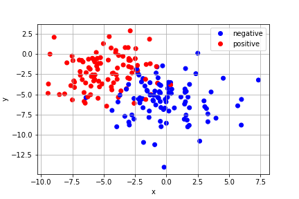
Consider a binary classification problem where we have data consisting of 3 parameters, \(\{(x,y,z)_i\}\), and a binary variable \(q_i\), taking values of 0 or 1, where \(i\) takes values 1 to \(n\). For example, \((x,y,z)_j\) might represent the location of the \(j\)th person in an apartment complex and \(q_j\) might represent whether or not they test positive for an infectious disease. The data may be clustered or grouped with respect to the category, or it may not. Below is an example where the data exhibit two clusters:

A human can easily make a qualitative judgement and draw a line (or a plane) separating the infected and uninfected clusters. We would like to see if we can let our computer do this through a fitting routine.

A plane may be specified by a normal unit vector \(\hat{\mathbf{n}}\) and a point \(\mathbf{p}\). Every point \(\mathbf{r}\) in the plane satisfies

\[\hat{\mathbf{n}}\cdot(\mathbf{r}-\mathbf{p}) = 0.\]

Since there are infinite choices for \(\mathbf{p}\), and \(\mathbf{r}\) is arbitrary, \((\mathbf{r}-\mathbf{p})\) could be any vector in the plane, and then this simply says that any vector lying in the plane must be perpendicular to \(\hat{\mathbf{n}}\). But most importantly for points to one side of the plane, we have

\[\hat{\mathbf{n}}\cdot(\mathbf{r}-\mathbf{p}) > 0,\]

and to the other side we have

\[\hat{\mathbf{n}}\cdot(\mathbf{r}-\mathbf{p}) < 0.\]

This behavior is just what we want to plug into some approximately binary function and model the classification problem. A good choice for a smooth approximately binary model is the logistic function:

\[h(z) = \frac{1}{1+e^{-z}}.\]

Over most of the real line this function is approximately 0 (at \(z\to -\infty\)) or 1 (as \(z\to + \infty\)) and it "turns on" in the region near \(z=0\). If we let

\[z(\mathbf{r}) = \hat{\mathbf{n}}\cdot(\mathbf{r}-\mathbf{p}),\]

then we see that \(h(z(\mathbf{r}))\) will be approximately 0 to one side of the plane and 1 to the other.

Since we don't know a priori what \(\hat{\mathbf{n}}\) or \(\mathbf{p}\) should be (at least not without doing the computer's job), we may as well call \(-\hat{\mathbf{n}}\cdot\mathbf{p} = \beta_0\). With these definitions

\[\hat{\mathbf{n}}\cdot(\mathbf{r}-\mathbf{p}) = \hat{\mathbf{n}}\cdot\mathbf{r}+\beta_0,\]

we see that the appropriate classifying function is

\[h(z) = \frac{1}{1+e^{-\hat{\mathbf{n}}\cdot\mathbf{r}-\beta_0}}.\]

One final modification is that we need to allow for the width of the turn on region to be adjusted. This means that we should allow the normal vector for the plane to be of any length, giving the usual form for the logistic function:

\[h(\beta_i,x_i) = \frac{1}{1+e^{-\beta_0-\beta_i x_i}},\]

with Einstein summation over the spatial indices \(i\).

Let's see how this model performs using lmfit to fit some clustered data generated with scikit-learn: